Mediation Analyses

Conducting simple mediation analyses in R

Introduction

In this tutorial, we will give a preliminary introduction on how to conduct simple mediation analyses in R. We will focus on running multiple regression analyses manually, to explain the concept of mediation and how to test for its significance. In practice, it is often recommended to use specialized packages for mediation analyses, but to develop a good intuition for the concept, you should first understand the basics.

What is mediation?

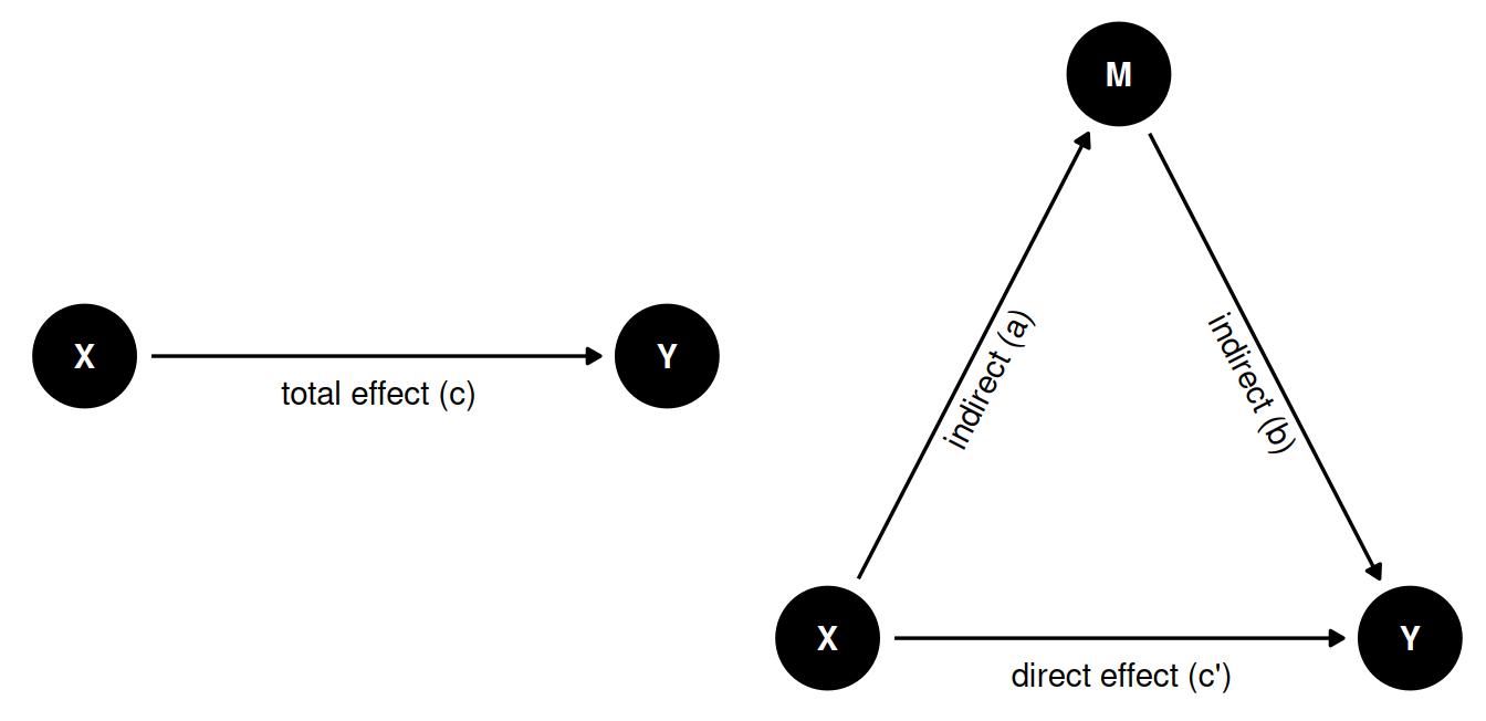
We are often interested in explaining a relationship or causal effect between two variables (e.g., X and Y). Many theories suggest that X does not necessarily directly influence Y, but that this effect is mediated by a third variable, which we can call M (for Mediation). We can visualize this interplay between the three variables like so:

In the left figure we see the total effect of X on Y. Here we only have one path from X to Y. In mediation analysis, the total effect is referred to as c.

In the right figure, we see a mediation model, where the effect of X on Y is mediated by M. This gives us two different paths for how X to have an effect on Y:

direct effect. The direct path X -> Y, referred to as c’.
indirect effect. The indirect path X -> M and M -> Y, referred to as a and b respectively. We can calculate the indirect effect by multiplying both arrows (a * b)

The mediated model can help us distinguish between different scenarios:

Full mediation: Only the indirect effect (a * b) is significant.
No mediation: Only the direct effect (c’) is significant.
Partial mediation: Both the direct and indirect effects are significant
No effect: Neither the direct nor the indirect effect is significant.

Note of caution: Theoretically, mediation models almost always suggest some sort of “causal chain”. Yet, the analysis itself cannot prove causality. The same caution applies as discussed in the causality section.

Packages and simulated data

library(tidyverse)
library(sjPlot)

For this tutorial we are going to simulate some data that align with the Figure presented above. You don’t need to understand this process, and can just run the code to create the data.

set.seed(42)
n <- 500
X <- rnorm(n, mean=3, sd=1)
M <- 0.5*X + rnorm(n, 0, 2)
Y <- 0.3*M + 0.8*X + rnorm(n, 0, 3)

d <- tibble(X,M,Y)

If you want to know how this simulation works

Here is a brief explanation of the data simulation code:

A seed is a starting point of the random number generator. Think of a random process in a computer as a jump in a random direction: as long as you’re starting point is the same, you’ll end up in the same place. By setting a specific seed, we thus ensure that the random data we generate is the same for everyone running this code. The number 42 is a common but arbitrary choice (it’s a pop-culture reference)
Create a random variable X that is normally distributed (mean = 3, sd = 1).
Create a variable M that is based on X, but with random noise. Note that we’re actually using the regression equation here. With 0.5*X we say that for every unit increase in X, M should go up by 0.5 (so \(b = 0.5\))). With rnorm(n, 0, 2) we add a residual (mean = 0, sd = 2) to the equation. We could also have added an intercept, but we left it out for sake of simplicity.
Create a random variable Y that is based on M (\(b = 0.3\)) and X (\(b = 0.8\)), with random noise.
This gives us a data set in which X influences Y both directly and indirectly through M.

Simple regression analyses

Let’s first look at the model without the mediator M.

m_total <- lm(Y ~ X, data = d)
tab_model(m_total)

	Y
Predictors	Estimates	CI	p
(Intercept)	-0.48	-1.32 – 0.36	0.263
X	1.06	0.80 – 1.33	<0.001
Observations	500
R² / R² adjusted	0.109 / 0.107

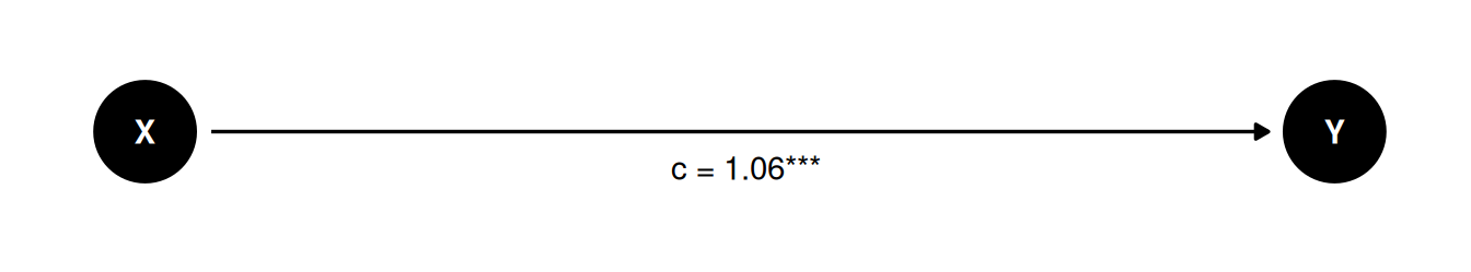
This gives us the total effect of X on Y.

Now let’s look at the model with the mediator M. We can break this model down into two separate regression models:

Model 1: M predicted by X.
Model 2: Y predicted by X and M.

m1 <- lm(M ~ X, data = d)
m2 <- lm(Y ~ X + M, data = d)

tab_model(m1, m2)

	M			Y
Predictors	Estimates	CI	p	Estimates	CI	p
(Intercept)	0.01	-0.57 – 0.59	0.973	-0.48	-1.30 – 0.34	0.250
X	0.48	0.30 – 0.67	<0.001	0.92	0.65 – 1.19	<0.001
M				0.30	0.18 – 0.43	<0.001
Observations	500			500
R² / R² adjusted	0.049 / 0.047			0.148 / 0.145

Let’s visualize the paths in the mediation model:

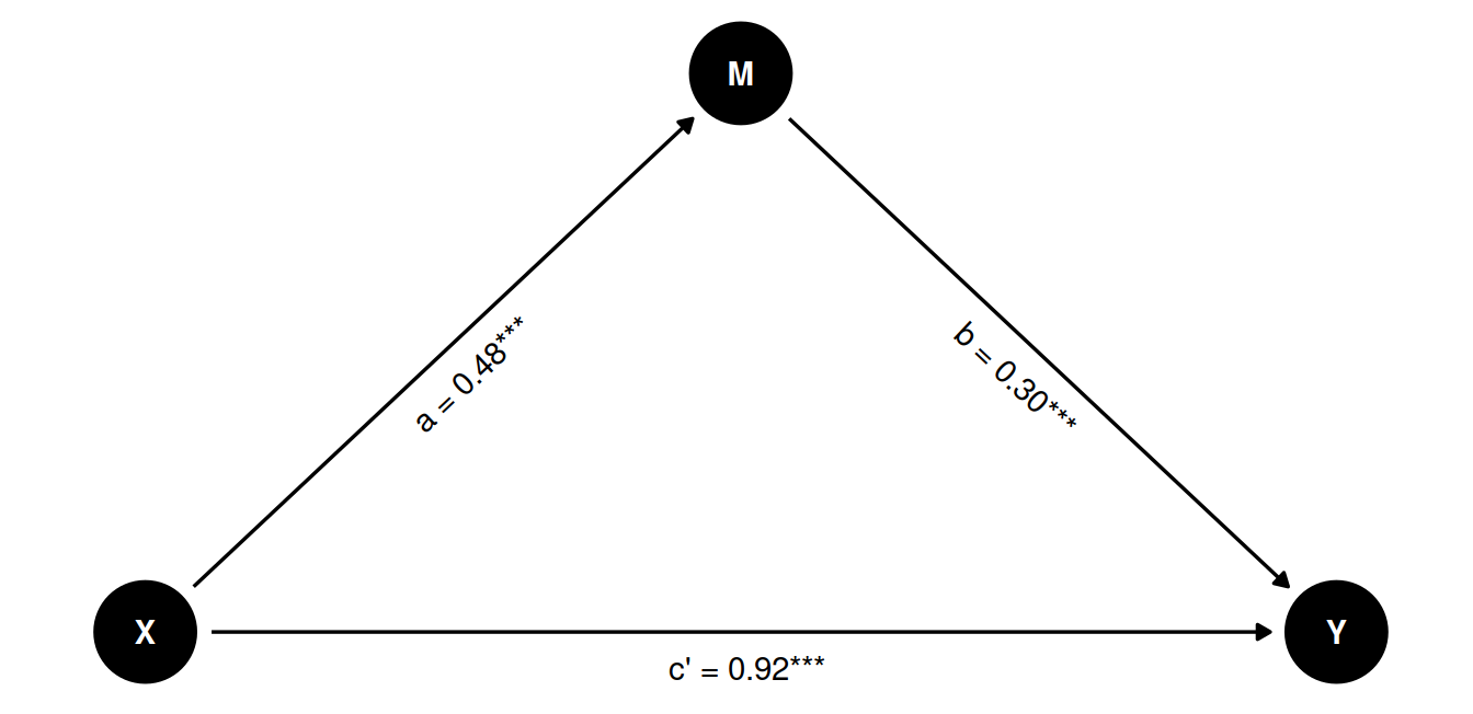
We can see that all paths are significant, suggesting that there is both a direct and indirect effect of X on Y. In other words, this is a partial mediation.

We can calculate the indirect effect by multiplying the coefficients of the two paths:

\[a \times b = 0.482 \times 0.301 = 0.15\]

Testing the significance of the indirect effect using PROCESS

The indirect effect consists of two parts: a and b. We have shown that we can calculate the indirect effect by multiplying these two parts. But how can we calculate the confidence interval for this indirect effect, and test if it is significant?

Calculating the required confidence interval for the indirect effect properly is not straightforward, and requires more advanced techniques like bootstrapping or Monte Carlo simulations, that we won’t cover here. Instead, we will show you how to use PROCESS in R, using the bruceR package. This will basically perform the same steps we did above, fitting three regression models to calculate the total, direct, and indirect effects. But in addition, it will also provide a confidence intervals based on bootstrapping.

To use PROCESS, you simply provide the data frame, and specify the column names for the dependent variable (y = "Y"), the independent variable (x = "X"), and the mediator (meds = "M"). The output might seem overwhelming at first, but if you look through it you should recognize the same components as we discussed before. The Model Summary shows the three regression models. The Part 2. Mediation/Moderation Effect Estimate shows the total (c), direct (c’) and indirect (a * b) effects. If you compare the effect sizes with the ones we calculated manually, you will see that they are the same. But the confidence intervalls are different, and we also get a confidence interval for the indirect effect.

library(bruceR)

PROCESS(d, y="Y", x="X", meds="M")


****************** PART 1. Regression Model Summary ******************

PROCESS Model Code : 4 (Hayes, 2018; www.guilford.com/p/hayes3)
PROCESS Model Type : Simple Mediation
-    Outcome (Y) : Y
-  Predictor (X) : X
-  Mediators (M) : M
- Moderators (W) : -
- Covariates (C) : -
-   HLM Clusters : -

All numeric predictors have been grand-mean centered.
(For details, please see the help page of PROCESS.)

Formula of Mediator:
-    M ~ X
Formula of Outcome:
-    Y ~ X + M

CAUTION:
  Fixed effect (coef.) of a predictor involved in an interaction
  denotes its "simple effect/slope" at the other predictor = 0.
  Only when all predictors in an interaction are mean-centered
  can the fixed effect denote the "main effect"!
  
Model Summary

──────────────────────────────────────────────────
             (1) Y        (2) M        (3) Y      
──────────────────────────────────────────────────
(Intercept)    2.684 ***    1.442 ***    2.684 ***
              (0.133)      (0.092)      (0.130)   
X              1.065 ***    0.482 ***    0.919 ***
              (0.137)      (0.095)      (0.137)   
M                                        0.301 ***
                                        (0.063)   
──────────────────────────────────────────────────
R^2            0.109        0.049        0.148    
Adj. R^2       0.107        0.047        0.145    
Num. obs.    500          500          500        
──────────────────────────────────────────────────
Note. * p < .05, ** p < .01, *** p < .001.

************ PART 2. Mediation/Moderation Effect Estimate ************

Package Use : ‘mediation’ (v4.5.0)
Effect Type : Simple Mediation (Model 4)
Sample Size : 500
Random Seed : set.seed()
Simulations : 100 (Bootstrap)

Running 100 simulations...
Indirect Path: "X" (X) ==> "M" (M) ==> "Y" (Y)
────────────────────────────────────────────────────────────
               Effect    S.E.     z     p      [Boot 95% CI]
────────────────────────────────────────────────────────────
Indirect (ab)   0.145 (0.043) 3.364 <.001 *** [0.065, 0.221]
Direct (c')     0.919 (0.123) 7.500 <.001 *** [0.732, 1.173]
Total (c)       1.065 (0.116) 9.147 <.001 *** [0.854, 1.285]
────────────────────────────────────────────────────────────
Percentile Bootstrap Confidence Interval
(SE and CI are estimated based on 100 Bootstrap samples.)

Note. The results based on bootstrapping or other random processes
are unlikely identical to other statistical software (e.g., SPSS).
To make results reproducible, you need to set a seed (any number).
Please see the help page for details: help(PROCESS)
Ignore this note if you have already set a seed. :)

Full mediation example

Full mediation

Since we’re working with simulated data, we can make a small adjustment to our code to simulate a scenario where M fully mediates the effect of X on Y. Notice that our simulation is almost identical, except that we set the coefficient of X on Y to 0.

set.seed(42)
n <- 500
X <- rnorm(n, 3, 1)
M <- 2*X + rnorm(n, 0, 2)
Y <- 0.3*M + 0*X + rnorm(n, 0, 3)
d_full <- tibble(X,M,Y)

To nicely interpret the models side-by-side, we’ll add some labels and drop the confidence intervals.

m_total <- lm(Y ~ X, data=d_full)
m1 <- lm(M ~ X, data=d_full)
m2 <- lm(Y ~ X + M, data=d_full)
tab_model(m_total, m1, m2,  
          dv.labels=c("Y ~ X", "M ~ X", "Y ~ X + M"), show.ci = FALSE)

	Y ~ X		M ~ X		Y ~ X + M
Predictors	Estimates	p	Estimates	p	Estimates	p
(Intercept)	-0.48	0.263	0.01	0.973	-0.48	0.250
X	0.71	<0.001	1.98	<0.001	0.12	0.522
M					0.30	<0.001
Observations	500		500		500
R² / R² adjusted	0.052 / 0.050		0.465 / 0.464		0.094 / 0.090

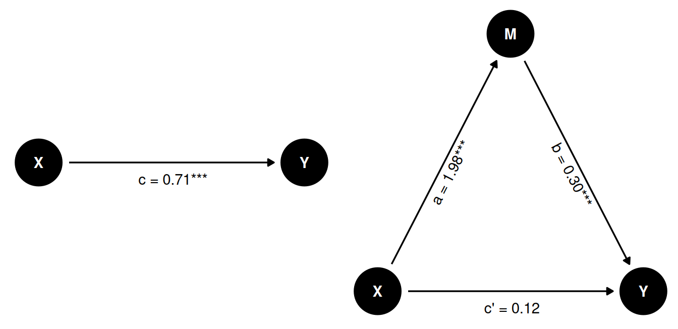
Here we do have an effect of X on Y, but when we control for M, the effect of X on Y is no longer significant. Since both the effect of X on M and M on Y are significant, this is a case of full mediation.

No mediation example

No mediation

We can also simulate a scenario where M has no effect on Y. We do not make the effect of M on Y zero, but we set the coefficient to a very small value, so that it is not significant.

set.seed(42)
n <- 500
X <- rnorm(n, 3, 1)
M <- 0.5*X + rnorm(n, 0, 2)
Y <- 0.05*M + 0.8*X + rnorm(n, 0, 3)
d_no_mediation <- tibble(X,M,Y)

m_total <- lm(Y ~ X, data=d_no_mediation)
m1 <- lm(M ~ X, data=d_no_mediation)
m2 <- lm(Y ~ X + M, data=d_no_mediation)
tab_model(m_total, m1, m2,  
          dv.labels=c("Y ~ X", "M ~ X", "Y ~ X + M"), show.ci = FALSE)

	Y ~ X		M ~ X		Y ~ X + M
Predictors	Estimates	p	Estimates	p	Estimates	p
(Intercept)	-0.48	0.250	0.01	0.973	-0.48	0.250
X	0.94	<0.001	0.48	<0.001	0.92	<0.001
M					0.05	0.414
Observations	500		500		500
R² / R² adjusted	0.091 / 0.089		0.049 / 0.047		0.092 / 0.089

In this case, the effect of X on Y is significant, but the effect of X on M is not. So there is no mediation effect. The full effect of X on Y is direct.